Seer3D 2

Seer3D^TM is an application for the visualization of field measurement data and the groundwater model results. It includes powerful tools for displaying vector and raster maps, presenting wells, boreholes, lithological, and geophysical data. Showcase your work by merging maps, field data and model results into stunning beautiful 3D scenes! Use the intuitive display control tools to emphasize displayed objects by adjusting their transparency and display types between mesh and solid, cropping objects with on-screen crop tools, and adding annotation, logo, and legend. Create animation videos of plume development, water level changes, flow vector field, and flow paths based on measurement data and model results. Advanced View feature enables you to store arbitrary view points and navigate between them. Present your models with eye-popping 3D stereoscoping display using Quad buffered stereo technology and deliver your Seer3D models with the free Seer3D viewer to your clients for great impression.

The main features of Seer3D are outlined below. Here are links to the user guide, free Seer3D Viewer, and sample models.

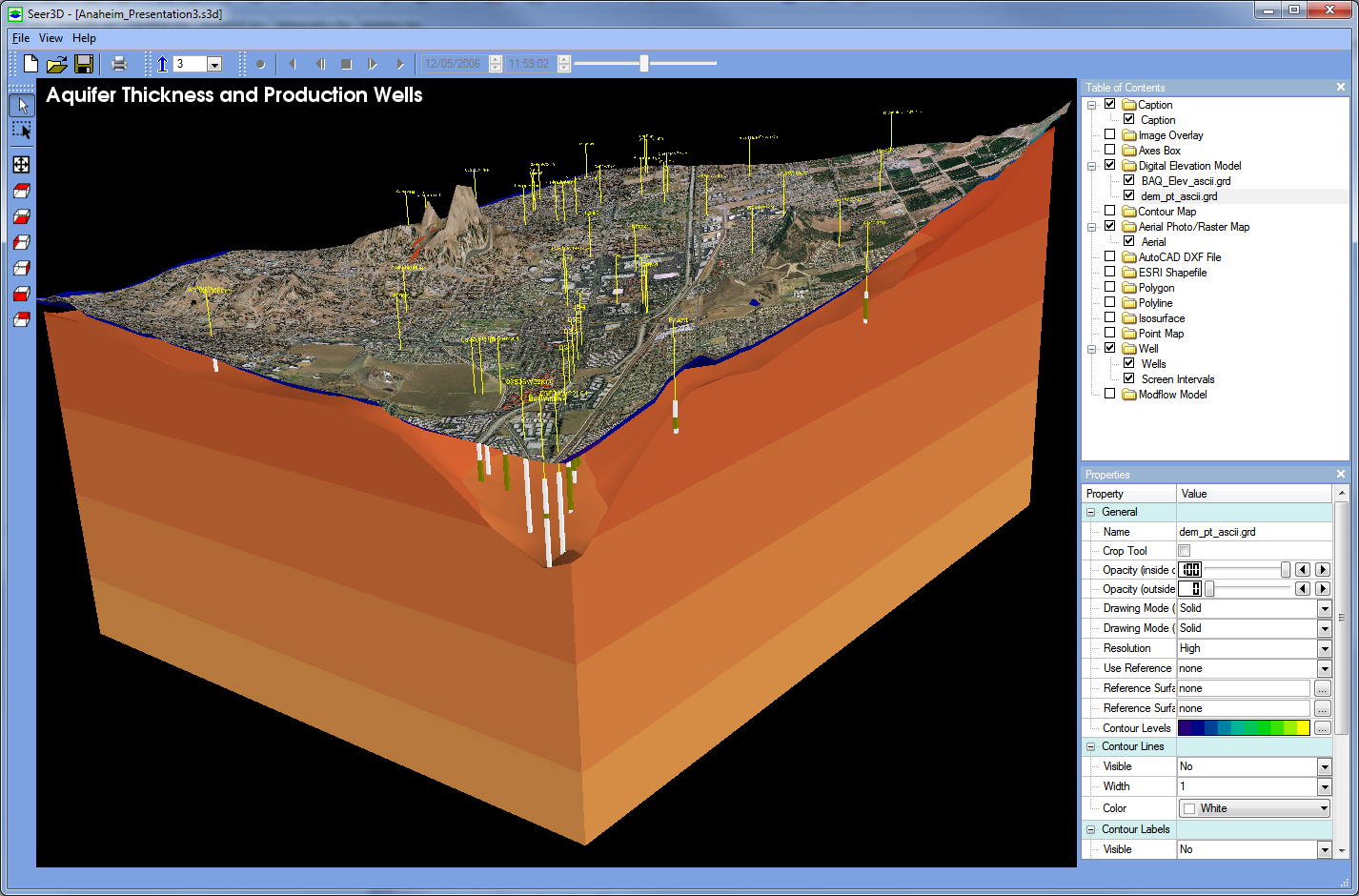
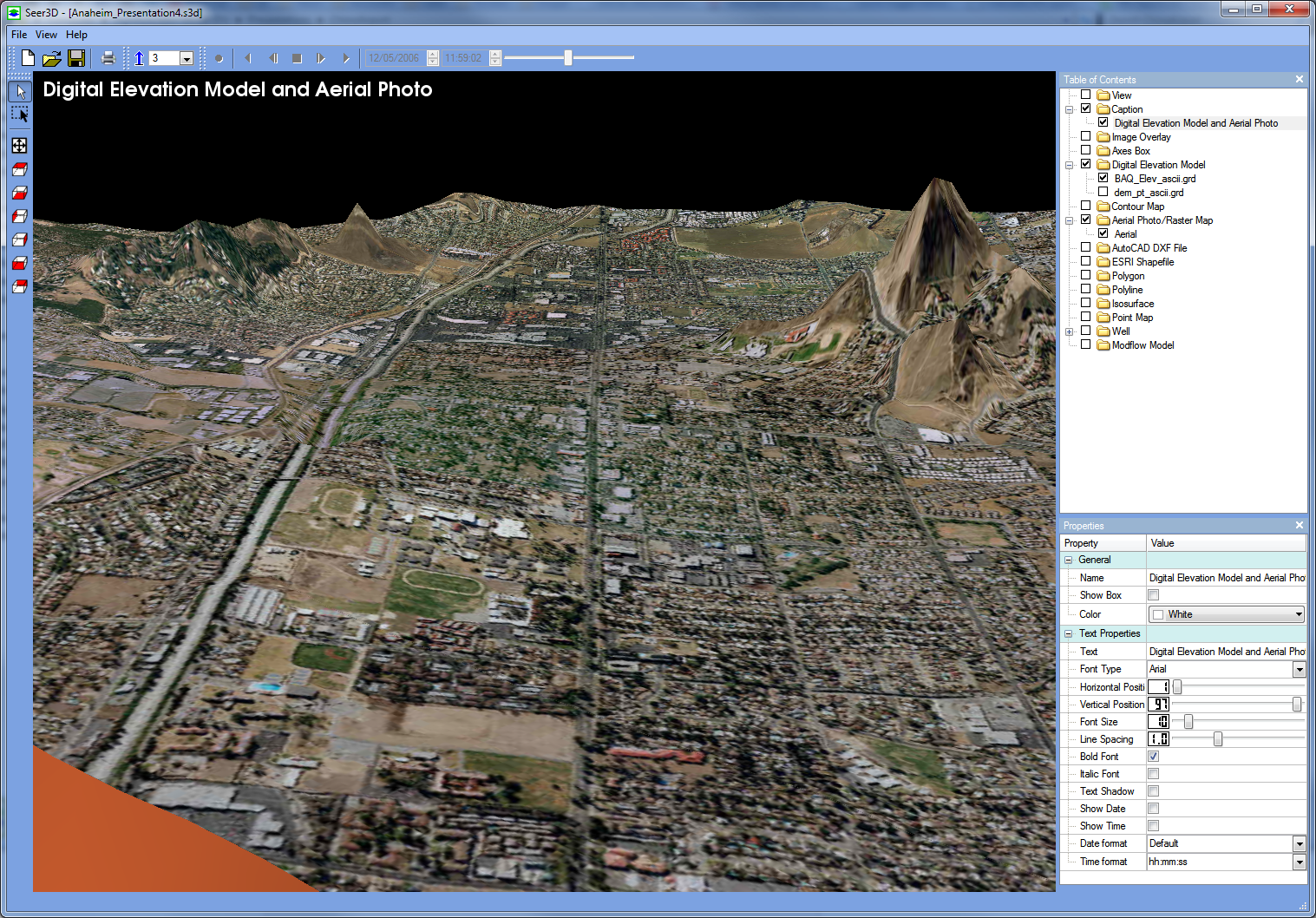
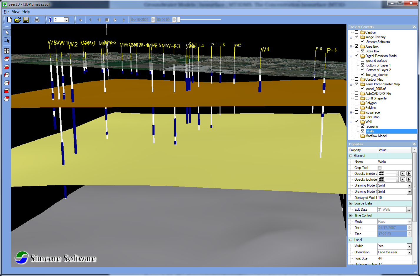
Digital Elevation Model & Aerial Photographs

• Digital Elevation Model (DEM) is a digital representation of ground surface topography or terrain based on a raster of elevation values. Seer3D supports several DEM formats, including Raster DEM (also known as ESRI ASCII Grid), SURFER Grid, SDTS DEM, and the GridFloat format of the National Elevation Dataset.
• Aerial Photographs can be georeferenced and draped on flat planes or on digital elevation models or contour maps to create photo-realistic terrain models. Seer3D supports aerial photographs that are save in PNG, JPG, TIF, or TIFF formats.

Numerical Models

Seer3D supports the USGS groundwater flow model MODFLOW, the transport models MT3DMS and SEAWAT, and a number of reactive transport models such as MT3D99, PHT3D, and RT3D. Seer3D can be used with most popular MODFLOW Graphical user interface applications, such as Processing Modflow, as long as they generate standard MODFLOW input datasets. The major features of the model support are outlined below:

• Model Grid: Displays the model grid.
• Flow Packages: Displays the model cells of the supported flow packages, such as river, drain, well, unsupported packages are ignored.
• Groundwater Table: Displays the simulated groundwater table in the form of color-filled contours.
• Hydraulic Head Contours: Displays simulated hydraulic heads in the form of color-filled contours on vertical or horizontal slices.
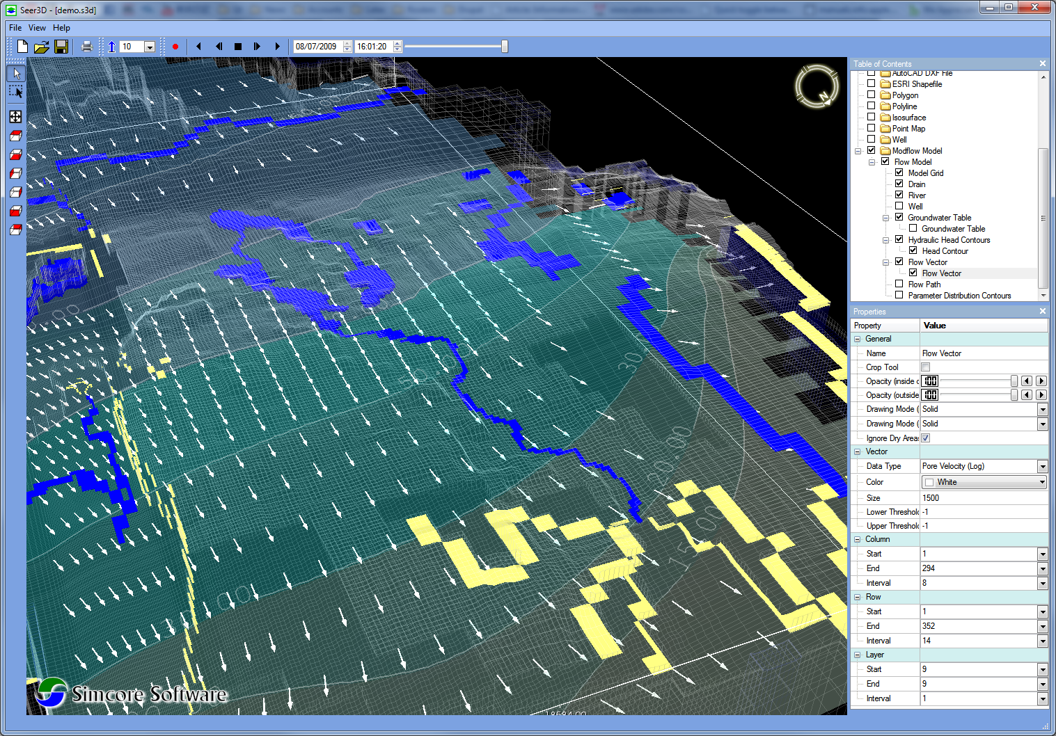
• Flow Vector Field: Display flow vector fields with flow vectors attached to model cells. The magnitude and direction of flow vectors are calculated based on the effective porosity and the simulated cell-by-cell flow terms and hydraulic head values.
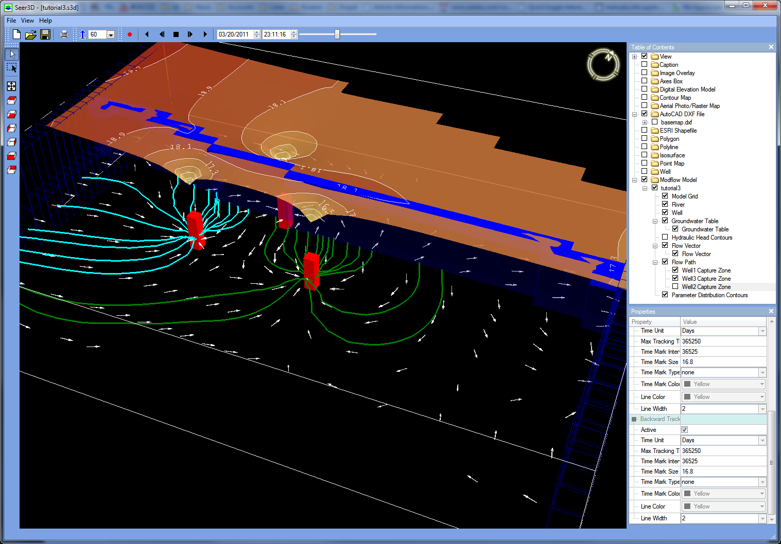
• Flow Path: Seer3D uses a semi-analytical particle-tracking scheme to calculate streamlines or pathlines based on the calculated hydraulic head values, the calculated cell-by-cell flow terms, and the starting locations and release times of particles.
• Concentration Contour: Displays simulated concentration values in the form of color-filled contours on vertical or horizontal slices.
• Concentration Isosurface: Displays simulated concentration values in the form of isosurface.
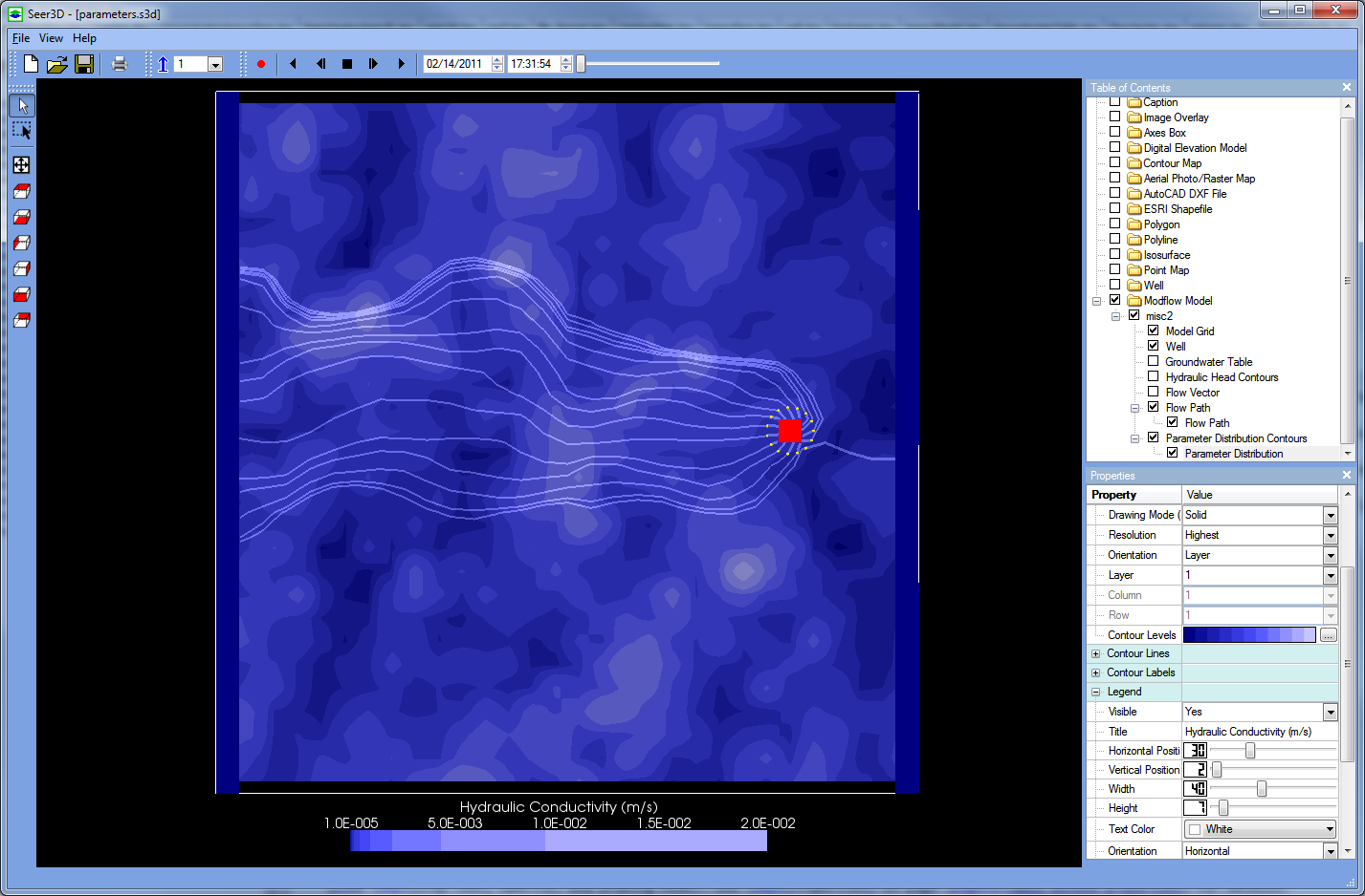
• Parameter Distribution: Displays spatial distribution of model parameter values, such as hydraulic conductivity, in the form of contours on vertical or horizontal slices.

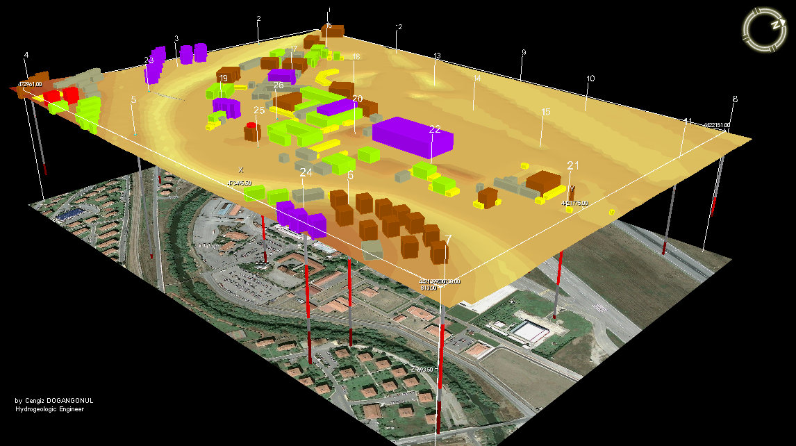
Vector Graphics

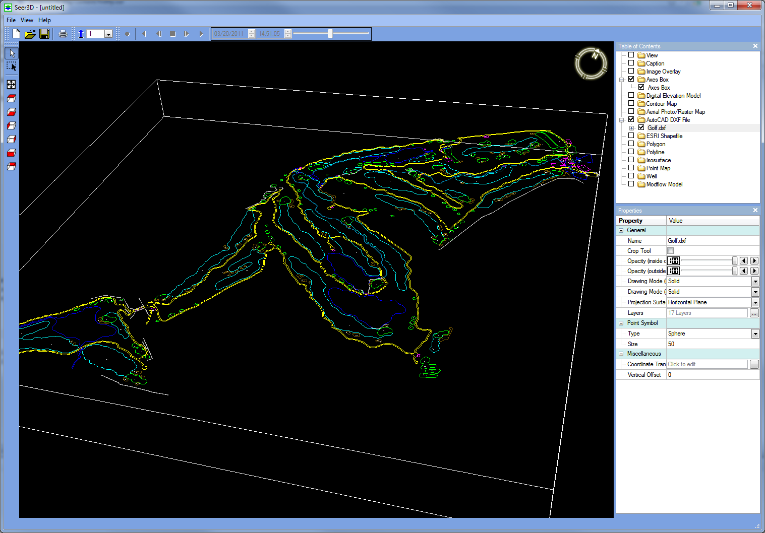
• DXF (Drawing eXchange Format): DXF is developed Autodesk for enabling data interoperability between AutoCAD and other programs. A DXF file contains all the information of an AutoCAD drawing file, including data of various types of graphical objects. Seer3D support the following graphical object types: POINT, LINE, POLYLINE, LWPOLYLINE, ARC, CIRCLE, SOLID, TEXT, MTEXT.
• Shapefile: The shapefile format is developed by ESRI as an open specification for data interoperability between software products of ESRI and other vendors. For example, you can import most results of Rockworks 15 via shapefiles, including solid layers, wells with stratigraphy, wells with lithology, fratures, geophysics, stratigraphic diagrams, etc.
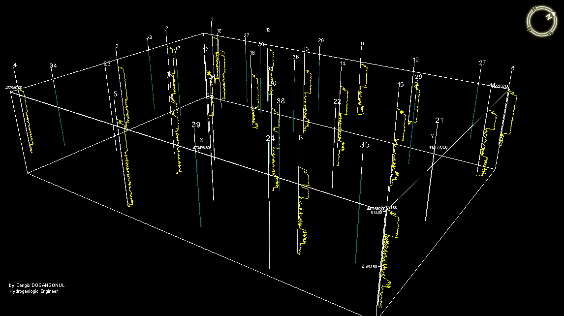
• Polyline: Polylines are simple and yet powerful features that are useful in many ways beyond drawing flow paths and boundary lines. For example, you can use polylines to display geophysical data next to well boreholes or display sparklines next to measurement points to present trends and variations of measurement data.
• Polygon: Polygons are primitive features that find many applications. For example, you can use polygons to display cross-sections of geological layers, or you can use complex polygons along with textures to display buildings.
• Wells: Display well casings, screen intervals, and lithology logs. You can import well data from files or from Microsoft Excel, Access,or SQL database through the built-in Open Database Connectivity (ODBC) interface. Slanted wells are supported by specifying the azimuth, inclination, and length of individual well segments.

Scattered Dataset

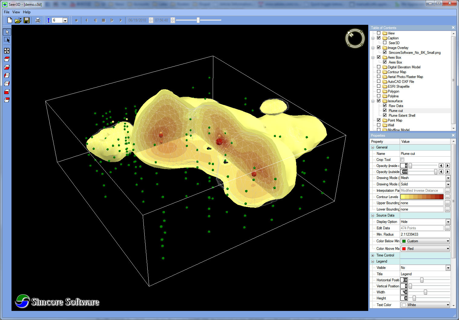
Scattered datasets in the form of (x, y, z, value, time) can be used by Seer3D to generate images and videos. You can import data from files or from Microsoft Excel, Access, or SQL database through the built-in Open Database Connectivity (ODBC) interface. The imported data can be represented in the following forms:

• Point Map: This displays point symbols with user-defined labels.
• Contour Map: Seer3D interpolates the elevations (z) and values of a scattered dataset to a 2D rectilinear grid and then create color-filled contours with labels that follow contour lines nicely. The elevation of the data points are interpolated so your contour maps do not necessarily need to lie on a flat plane, but on a surface based on the interpolated elevation values. You can customize the display by modifying the interpolation parameters, contour levels, and color ramp, etc. You can also create animated contour maps if the scattered dataset contains the temporal information (time).
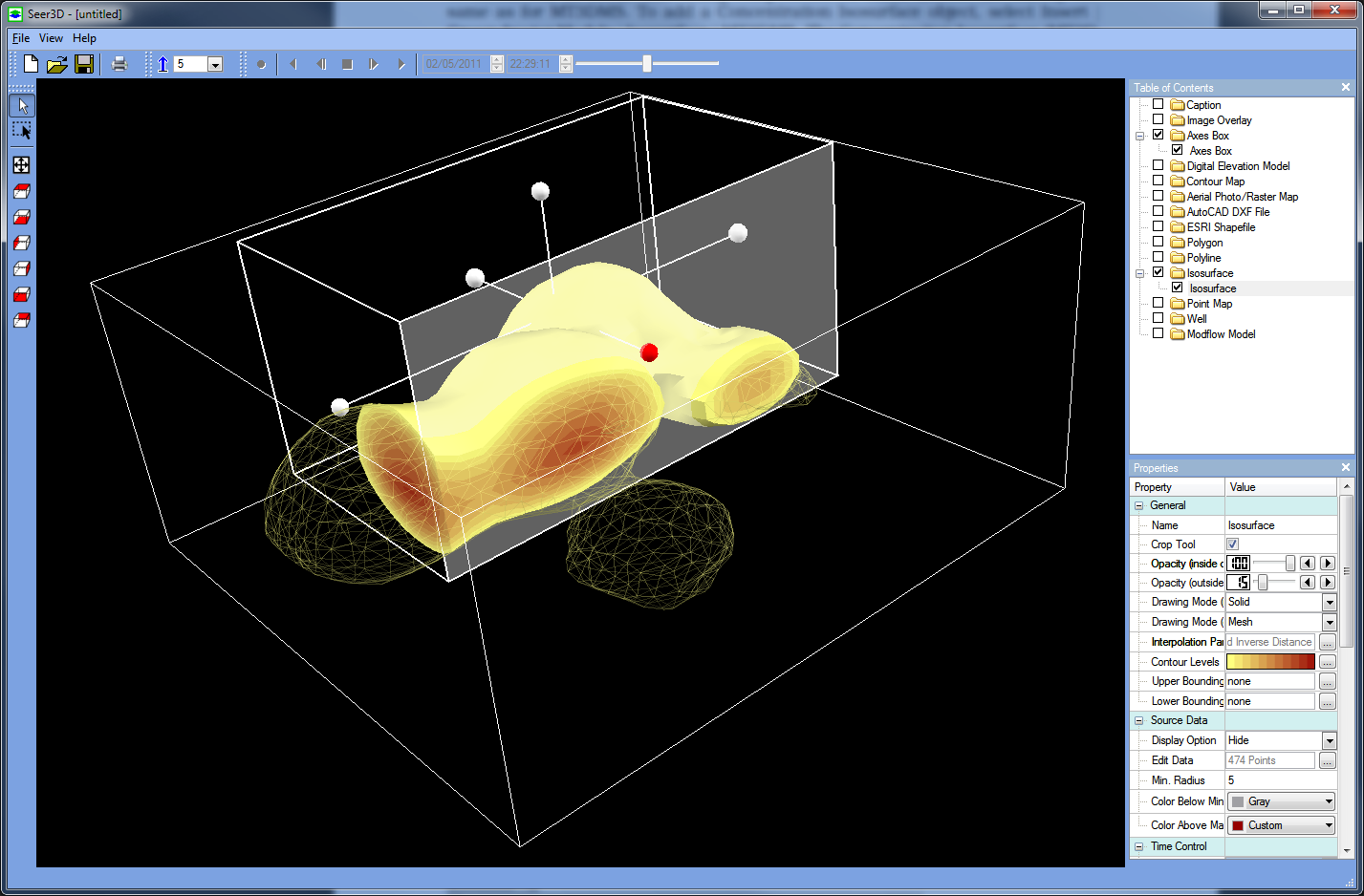
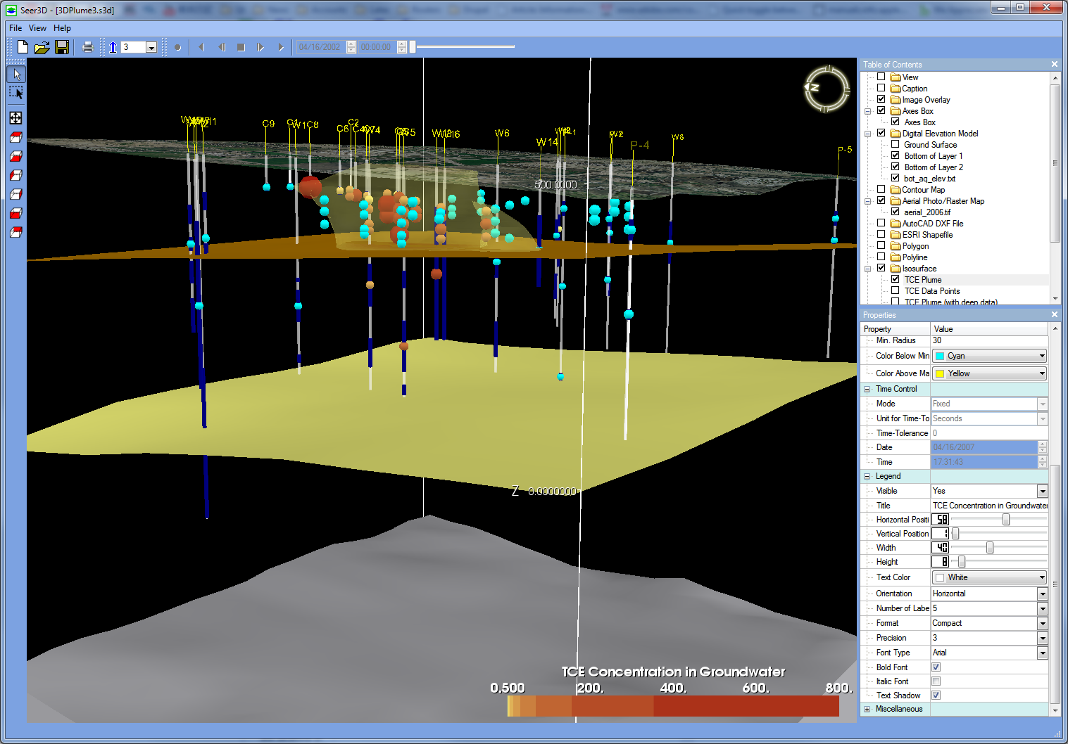
• Isosurface: Seer3D interpolates the values of a scattered dataset to a 3D rectilinear grid and then create an isosurface of a given value. You can use the built-in crop tool to cut through the isosurface and to display the distribution of interpolated values inside the isosurface in the form of color-filled contours. Similar to the Contour Map, you can modify a number of display settings and create animated isosurface if the scattered dataset contains the temporal information (time).

System Requirements

The minimum requirements are given below. Please see the user guide for the recommended Configuration for Quad-Buffered 3D Stereographic Display.

• Operating System: Microsoft Windows XP, Windows 7 (32 or 64 bit), Windows 10 (32 or 64 bit).
• CPU: Pentium 4, 2.4 GHz+ or AMD 2400xp+
• System Memory (RAM): 2 GB
• Hard Disk: 1GB of free disk space
• Graphics Card: OpenGL-capable card with 256 MB of Video RAM or greater (most 3D graphics cards will work with Seer3D) .
• 1280×1024, ”32-bit True Color” screen (most LCD panels are better than this).

Limitations

While Seer3D does not assume any constraints on the size of datasets or models, the application is still subject to limitations imposed by the complexity of loaded datasets and the operating system. As it is impractical to provide specific software limitation information, the following may give you an idea of whether Seer3D suits your needs: Seer3D has been used to display two groundwater models simultaneously along with a number of DEMs and aerial photographs. One of the loaded models was used for model calibration with data from the past decades and the other was used for predicting groundwater flows in the coming decades. Flow vectors of the models were displayed at at an interval of every six cells and at the first model layer. Streamlines were calculated and displayed for the second model. The dimension of those two models are approximately 550 x 550 x 3 x 220 (columns x rows x layers x stress periods).