This page contains a number of 3D Visualization models that are constructed by Seer3D. To visualize the models, you need to install Seer3D. Click here to download the Seer3D Setup. All models are based on fictitious data and are solely for demonstration purposes. Click next to the name of a model to display its screen shot.
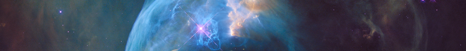
- Tutorial 1 (Last update: 5/9/2011; 55 KB): This Seer3D model visualize the MODFLOW model that is described in Section 4.1 of the user’s guide of Processing Modflow 8. The Seer3D model shows flow vectors, streamlines, groundwater level contours based on the result of the flow model. An AutoCAD DXF file overlays the model for orientation purposes. To use this model, download and unzip content of the tutorial1 file to a clean folder, and then open the unzipped tutorial1.s3d file.
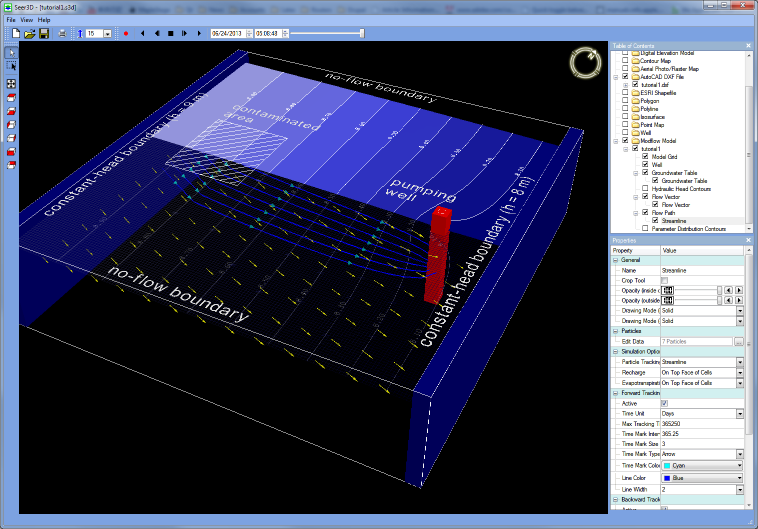
- Tutorial 2 (Last update: 5/9/2011; 260 KB): This Seer3D model visualize the MODFLOW model that is described in Section 4.2 of the user’s guide of Processing Modflow 8. The Seer3D model animates flow vectors and groundwater level contours based on the transient model result. To use this model, download and unzip the content of tutorial2 file to a clean folder, and then open the unzipped tutorial2.s3d file. Once the model is loaded, click on the Play Forward button to start animation.
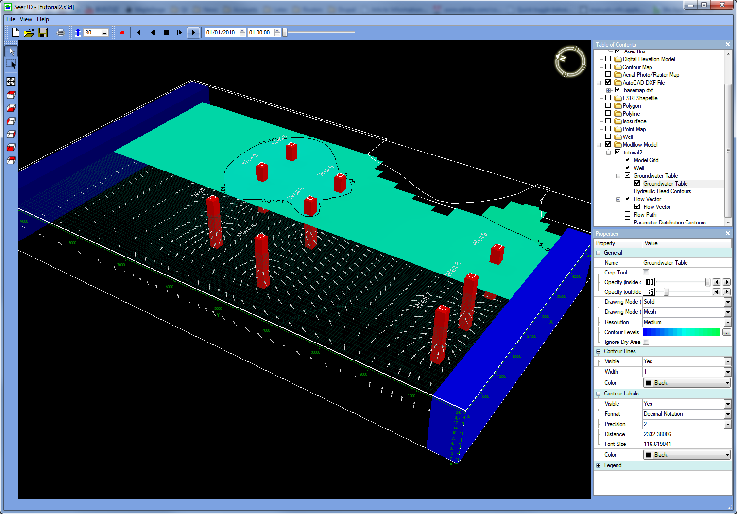
- Tutorial 3 (Last update: 5/9/2011; 71 KB): This Seer3D model visualize the MODFLOW model that is described in Section 4.3 of the user’s guide of Processing Modflow 8. The Seer3D model displays flow vectors, streamlines, and groundwater level contours based on the result of the flow model. Several “views” are stored in the Seer3D model that allowing users “flying” from one view point to another. To use this model, download and unzip the content of the tutorial3 file to a clean folder, and then open the tutorial3.s3d file. Once the model is loaded, right-click on any of the Views (View 1 through View 5) on the Table of Contents, and the select Go To to start animation.
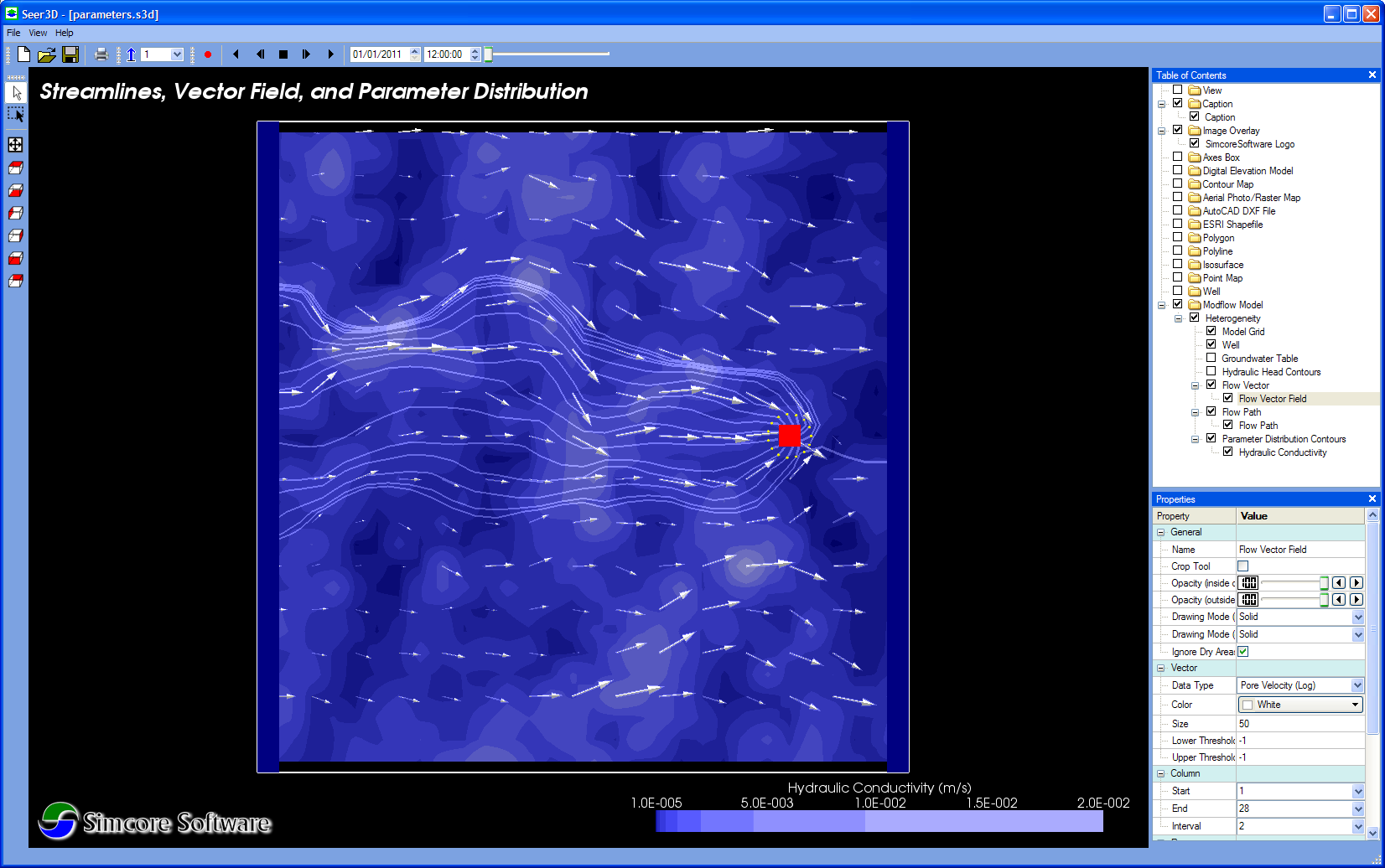
- Streamlines and vector field in a heterogeneous aquifer. (Last update: 6/2/2011; 50 KB): The groundwater flow field in a heterogeneous aquifer is simulated with MODFLOW. Seer3D displays the distribution of the hydraulic conductivity and vector field. The size of the vectors represents the magnitude of flow volume, pore velocity, or Darcy velocity. The streamlines are calculated by Seer3D with the starting points (yellow dots) set around the pumping well (red square). To use this model, download and unzip the content of parameters.zip to a clean folder, and then open the unzipped parameters.s3d file with Seer3D.
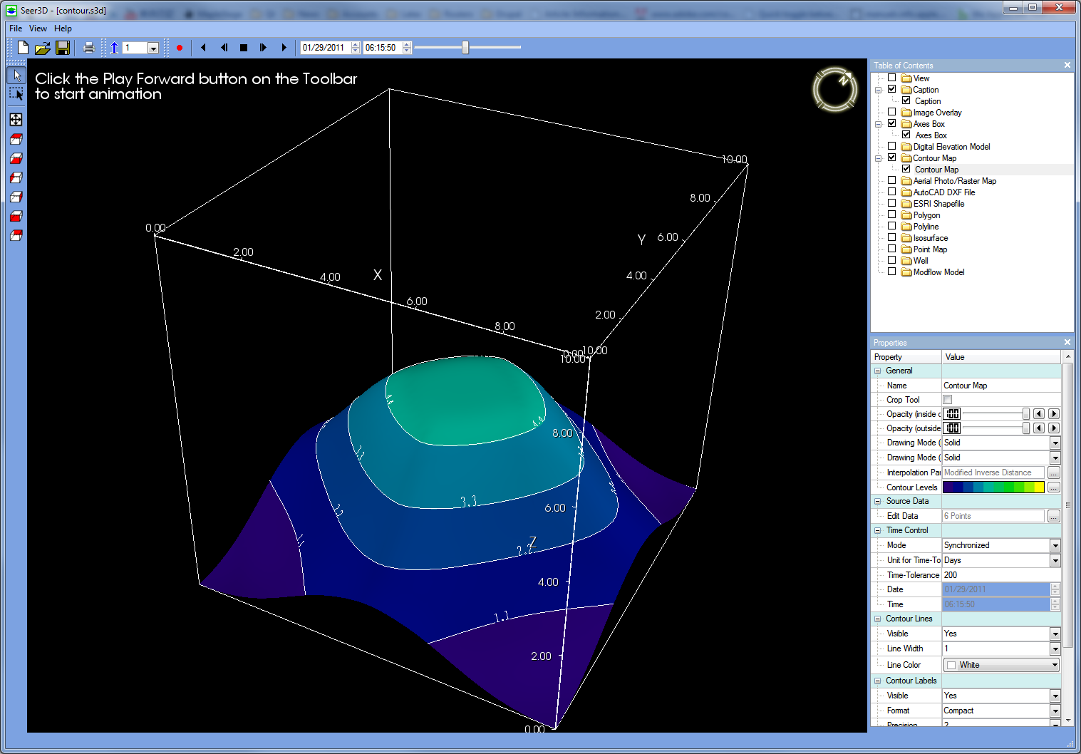
- Contour Map (Last update: 5/9/2011; 18 KB): This model demonstrates the contour map animation feature of Seer3D. The model contains a contour map based solely on 5 “measurement” points that are evenly distributed on a 10×10 square. The measured value of all 5 points is zero at the begining of the animation (1/1/2011). The measured value of the point located at the center of the square is 10 at the end of the animation (3/1/2011) while the measured values of the other points remain unchanged. The animation depicts the change of the contour map over time and is created by both spatial and temporal interpolation of the measured values. To use this model, download and open the contour.s3d file. Once the model is loaded, click on the Play Forward button to start animation.
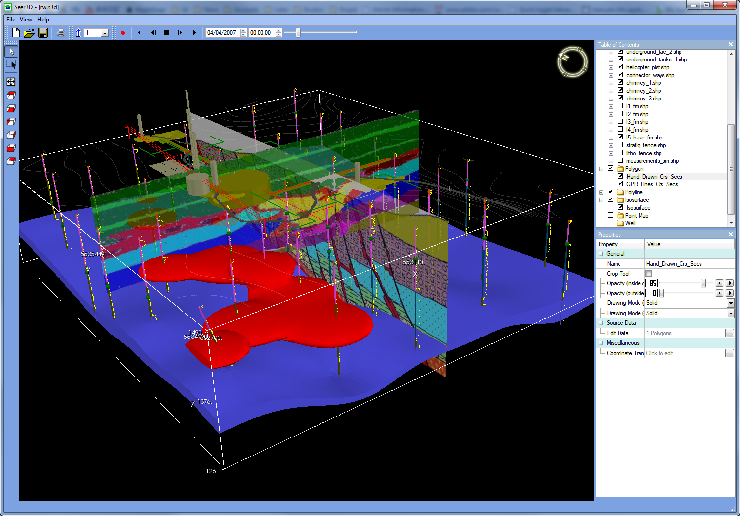
- Rockware/3D Shapefile (Last update: 5/9/2011; 7,862 KB): This Seer3D model, provided courtesy of Mr. Cengiz DOĞANGÖNÜL, demonstrates the capability of loading the models created by Rockworks via 3D Shapefiles, including geologic layers, geophysic data, fence diagrams, etc. In addition, this model displays a hand-drawn cross-section, a GPR (ground penetrating radar) cross-section, and a 3D isosurface of concentration measurements. To use this model, download and open the rw.s3d file. You can turn on a number of shapefiles that are not displayed by default.